Exercise 3: Join Cost Estimation
查询代价
exercise3要做的是估计连接查询的代价,以下是讲义:
其实这应该是四个exercise最容易的一个,就是看懂了连接查询的公式,然后写一下就好了,以下是公式:
scancost(t1) + scancost(t2) + joincost(t1 join t2) + scancost(t3) + joincost((t1 join t2) join t3) +
这里提一下基于成本的估计。
一般查询的成本分为I/O成本和CPU成本,I/O成本就是我们扫描表获取记录时,需要发生磁盘I/O,产生的时间成本为I/O成本;
而有了记录,我们需要判断这些记录符不符合查询的条件,这需要CPU去做,其中产生的时间就是CPU成本。
对于连接查询来说,以两表连接为例,首先需要扫描一张表然后过滤出一些记录,然后把过滤完的记录,每一条都去与第二张表进行匹配,这里第一张表称为驱动表t1,第二张表称为被驱动表t2。
在两表连接中,驱动表只需要扫描一次,然后产生card1条记录,而被驱动表则需要扫描card1次,这是总的IO成本;然后假设t2表有card2条记录,则产生的CPU成本应该为 card1 * card2。
所有总成本应该为:
t1的IO成本 + t1的记录数*t2的IO成本 (I/O成本) +t1的记录数*t2的记录数(CPU成本)
当然,实际的数据库去计算这些成本,都会有一些参数去调节,但总体的公式就是这样。
实现
根据公式写出来的代码:
public double estimateJoinCost(LogicalJoinNode j, int card1, int card2, double cost1, double cost2) {
    if (j instanceof LogicalSubplanJoinNode) {
        // A LogicalSubplanJoinNode represents a subquery.
        // You do not need to implement proper support for these for Lab 3.
        return card1 + cost1 + cost2;
    } else {
        // Insert your code here.
        // HINT: You may need to use the variable "j" if you implemented
        // a join algorithm that's more complicated than a basic
        // nested-loops join.
        final double IoCost = cost1 + card1 * cost2;
        final double CpuCost = card1 * card2;
        return IoCost + CpuCost;
    }
}
基数估计
做完这个之后,该exercise的另一个任务就是估计连接产生的基数(cardinality),也就是产生结果的记录数。
简单总结一下:
-
如果其中一个是非主键, 我们选择非主键的 card 作为 joinCard
-
如果两个都是非主键, 我们选择 最大的 card 作为 joinCard
-
如果两个都是主键, 我们选择最小的 card 作为 joinCard
为什么呢????????
有了上面的理论基础,就可以写出代码了:
public static int estimateTableJoinCardinality(Predicate.Op joinOp, String table1Alias, String table2Alias,
                                                   String field1PureName, String field2PureName, int card1, int card2,
                                                   boolean t1pkey, boolean t2pkey, Map<String, TableStats> stats,
                                                   Map<String, Integer> tableAliasToId) {
    /**
     * * For equality joins, when one of the attributes is a primary key, the number of tuples produced by the join cannot
     *   be larger than the cardinality of the non-primary key attribute.
     *
     * * For equality joins when there is no primary key, it's hard to say much about what the size of the output
     *   is -- it could be the size of the product of the cardinalities of the tables (if both tables have the
     *   same value for all tuples) -- or it could be 0.  It's fine to make up a simple heuristic (say,
     *   the size of the larger of the two tables).
     *
     * * For range scans, it is similarly hard to say anything accurate about sizes.
     *   The size of the output should be proportional to
     *   the sizes of the inputs.  It is fine to assume that a fixed fraction
     *   of the cross-product is emitted by range scans (say, 30%).  In general, the cost of a range
     *   join should be larger than the cost of a non-primary key equality join of two tables
     *   of the same size.
     */
    int card = 1;
    if (t1pkey && t2pkey) {
        card = Math.min(card1, card2);
    } else if (!t1pkey && !t2pkey) {
        card = Math.max(card1, card2);
    } else {
        card = t1pkey ? card2 : card1;
    }
    switch (joinOp) {
        case EQUALS: {
            break;
        }
        case NOT_EQUALS: {
            card = card1 * card2 - card;
            break;
        }
        default: {
            card = card1 * card2 / 3;
        }
    }
    return card <= 0 ? 1 : card;
}
Exercise 4: Join Ordering
exercise3我们完成了连接查询的成本估计与基数估计,而exercise4我们要做的是根据在多表连接的情况下,去选择一个最优的连接顺序,来实现对连接查询的优化。
有了这个连接顺序就可以生成执行计划了。
总体的思想是列举出所有的连接顺序,计算出每种连接顺序的代价,然后选择代价最小的连接顺序去执行。
但是,如何列举是个问题。
举个例子,对于两表连接,连接顺序有2 * 1种可能;对于三表连接,有3 * 2 * 1 = 6种可能。
可以发现,按照枚举的方式去弄,有n!种方案。当n = 7时,方案数有655280种;
当n = 10时,方案数可以达到176亿。
可以看到,这个缺点特别明显,就是当连接的表数一多,我们的方案数回很多,时间复杂度很高。
所以本实验采用的是一种基于动态规划的查询计划生成。
动态规划的思想, 相信大家都有所了解, 也即先将低纬度的给计算好, 然后让高纬度基于低纬度进行计算, 在本次实验中,
我们只关心 left-deep-tree
举个例子, 假设我们有四个表, 分别是: emp, dept, hobby, hobbies
我们想执行这个 sql 语句:
select xx from emp, dept, hobby, hobbies

where
hobbies.c1 = hobby.c0 and
emp.c1 = dept.c0 and
emp.c2 = hobbies.c0
如何计算这三个连接的顺序呢?
假设利用 node1 代表 hobbies.c1 = hobby.c0
node2 代表 emp.c1 = dept.c0
node3 代表 emp.c2 = hobbies.c0
-
第一步: 先计算 1 个 joinNode 的执行代价, 也即 sql 中的 hobbies join hobby, emp join dept …., 并将这三个代价保存到一个 costmap 中 -»> node1->cost , node2 -> cost, node3->cost
-
第二步, 计算 2 个 joinNode 的最优执行代价:
- 生成2个 joinNode 的不同顺序: (node1, node2), (node1, node3), (node2, node3) 共三种顺序
- 其中, 去除 (node1, node2), 因为这两个 node 没有交集, 也即不存在一个表, 同时出现在两个 node 中
- 分别计算 (node1, node3), (node2, node3) 的最优执行计划
- 以 (node1, node3) 为例, 我们可以选择让 (hobbies join hobby) join emp, 也可以选择让 (emp join hobbies) join hobby, 选择的依据就是哪个 cost 比较小 (这里可能不好理解, 因为多表join, 我们考虑的是 left-deep-tree, 也即是前面的 join 执行完后, 再和第三个表 join)
- 这一步之后, costmap就有了 (node1, node3) -> cost, (node2, node3) -> cost
- 同时, 还可以他们的最优执行顺序 planMap, 比如 (node1, node3) 的顺序可能是 (node3, node1)
-
第三步, 计算 3 个 joinNode 的最优执行计划
- 步骤和 第二步类似, 也是让两个 node 先 join, 再join 第三个 node
下面是实验讲义给出的动态规划法伪代码:
j = set of join nodes
for (i in 1...|j|):
     for s in {all length i subsets of j}
       bestPlan = {}
       for s' in {all length d-1 subsets of s}
            subplan = optjoin(s')
            plan = best way to join (s-s') to subplan
            if (cost(plan) < cost(bestPlan))
               bestPlan = plan
     optjoin(s) = bestPlan
return optjoin(j)
java 实现:
public List<LogicalJoinNode> orderJoins(Map<String, TableStats> stats, Map<String, Double> filterSelectivities,
                                        boolean explain) throws ParsingException {
    final PlanCache pc = new PlanCache();
    CostCard costCard = null;
    for (int i = 1; i <= this.joins.size(); i++) {
        // 生成 size = i 的子集, 可以利用回溯算法来做
        final Set<Set<LogicalJoinNode>> subsets = enumerateSubsets(this.joins, i);
        for (final Set<LogicalJoinNode> subPlan : subsets) {
            double bestCost = Double.MAX_VALUE;
            for (final LogicalJoinNode removeNode : subPlan) {

                // 尝试将这个子集中的一个 node 从该子集中去除, 然后子集中剩下的 joinNode 进行 join, 估算代价
                // 比如, node1 join node2 join node3
                // 我们去除了  node1 ,
                // 然后估算 (node2 join node3) join node1 和 node1 join (node2 join node3), 这两种哪个代价比较小, 而 (node2 join node3) 我们已经在之前的遍历中计算好了
                final CostCard cc = computeCostAndCardOfSubplan(stats, filterSelectivities, removeNode, subPlan,
                    bestCost, pc);
                if (cc != null) {
                    bestCost = cc.cost;
                    costCard = cc;
                }
            }
            // 保存该子集的最优执行计划
            if (bestCost != Double.MAX_VALUE) {
                pc.addPlan(subPlan, bestCost, costCard.card, costCard.plan);
            }
        }
    }
    if (costCard != null) {
        return costCard.plan;
    } else {
        return joins;
    }
}
computeCostAndCardOfSubplan 的逻辑如下:
这个函数的目的是为了计算处 card1, card2, cost1, cost2, 并通过这四个参数计算 join cost
举个例子, 如果 joinSet = (node1, node2, node3), removeNode = node3
-
首先构建一个 news, 去除了 removeNode, news = (node1, node2)
-
根据 News, 获取之前已经计算好的 bestPlan -> 也即顺序可能是 (node2 join node1)
-
如果 removeNode 的 table1 包含在 news 中, 那么计算的流程就是 (node2 join node1) join node3
-
card1 = news.card, cost1 = news.bestCost
-
card2 = table2.card, cost2 = table2.cost
-
-
同理, 如果 table2 包含在 news 中, 计算流程就是 node3 join (node2 join node1)
private CostCard computeCostAndCardOfSubplan(Map<String, TableStats> stats,
                                             Map<String, Double> filterSelectivities, LogicalJoinNode joinToRemove,
                                             Set<LogicalJoinNode> joinSet, double bestCostSoFar, PlanCache pc) throws ParsingException {
    LogicalJoinNode j = joinToRemove;
    List<LogicalJoinNode> prevBest;
    if (this.p.getTableId(j.t1Alias) == null)
        throw new ParsingException("Unknown table " + j.t1Alias);
    if (this.p.getTableId(j.t2Alias) == null)
        throw new ParsingException("Unknown table " + j.t2Alias);
    String table1Name = Database.getCatalog().getTableName(this.p.getTableId(j.t1Alias));
    String table2Name = Database.getCatalog().getTableName(this.p.getTableId(j.t2Alias));
    String table1Alias = j.t1Alias;
    String table2Alias = j.t2Alias;

    // 构建子集, 去除 removeNode
    Set<LogicalJoinNode> news = new HashSet<>(joinSet);
    news.remove(j);
    double t1cost, t2cost;
    int t1card, t2card;
    boolean leftPkey, rightPkey;
    if (news.isEmpty()) { // base case -- both are base relations
        // 如果news 为空 , 说明是 base case, 我们只需要计算 removeNode 的代价就可以了
        prevBest = new ArrayList<>();
        t1cost = stats.get(table1Name).estimateScanCost();
        t1card = stats.get(table1Name).estimateTableCardinality(filterSelectivities.get(j.t1Alias));
        leftPkey = isPkey(j.t1Alias, j.f1PureName);
        t2cost = table2Alias == null ? 0 : stats.get(table2Name).estimateScanCost();
        t2card = table2Alias == null ? 0 : stats.get(table2Name).estimateTableCardinality(
            filterSelectivities.get(j.t2Alias));
        rightPkey = table2Alias != null && isPkey(table2Alias, j.f2PureName);
    } else {
        // 如果不为空, 先取出 news 的最优执行计划, 包括执行顺序和代价
        prevBest = pc.getOrder(news);
        // possible that we have not cached an answer, if subset
        // includes a cross product
        if (prevBest == null) {
            return null;
        }
        double prevBestCost = pc.getCost(news);
        int bestCard = pc.getCard(news);
        // 如果 removeNode 的 left 包含在 prevBest 中
        // 那么 card1 = news 的 bestCard
        if (doesJoin(prevBest, table1Alias)) { // j.t1 is in prevBest
            t1cost = prevBestCost; // left side just has cost of whatever
                                   // left
            // subtree is
            t1card = bestCard;
            leftPkey = hasPkey(prevBest);
            t2cost = j.t2Alias == null ? 0 : stats.get(table2Name).estimateScanCost();
            t2card = j.t2Alias == null ? 0 : stats.get(table2Name).estimateTableCardinality(
                filterSelectivities.get(j.t2Alias));
            rightPkey = j.t2Alias != null && isPkey(j.t2Alias, j.f2PureName);
        } else if (doesJoin(prevBest, j.t2Alias)) { // j.t2 is in prevbest
                                                    // (both
            // shouldn't be)
            t2cost = prevBestCost; // left side just has cost of whatever
                                   // left
            // subtree is
            t2card = bestCard;
            rightPkey = hasPkey(prevBest);
            t1cost = stats.get(table1Name).estimateScanCost();
            t1card = stats.get(table1Name).estimateTableCardinality(filterSelectivities.get(j.t1Alias));
            leftPkey = isPkey(j.t1Alias, j.f1PureName);
        } else {
            // don't consider this plan if one of j.t1 or j.t2
            // isn't a table joined in prevBest (cross product)
            return null;
        }
    }

    // 计算 join 代价
    double cost1 = estimateJoinCost(j, t1card, t2card, t1cost, t2cost);
    LogicalJoinNode j2 = j.swapInnerOuter();
    double cost2 = estimateJoinCost(j2, t2card, t1card, t2cost, t1cost);
    if (cost2 < cost1) {
        boolean tmp;
        j = j2;
        cost1 = cost2;
        tmp = rightPkey;
        rightPkey = leftPkey;
        leftPkey = tmp;
    }
    if (cost1 >= bestCostSoFar)
        return null;
    CostCard cc = new CostCard();
    cc.card = estimateJoinCardinality(j, t1card, t2card, leftPkey, rightPkey, stats);
    cc.cost = cost1;
    cc.plan = new ArrayList<>(prevBest);
    cc.plan.add(j); // prevbest is left -- add new join to end
    return cc;
}
我们可以对比一下优化前后提高的速度。
优化前默认的连接顺序:耗时5s645ms
优化后选择了最佳的连接顺序:耗时1s673ms
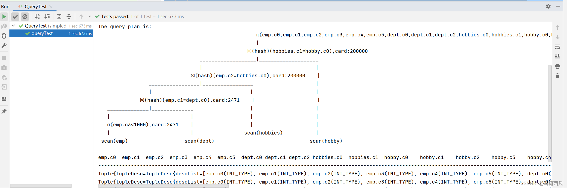
可以看到,速度快了三倍。
可见查询优化是多么重要。
小结
我们想要获取更好的概率,那么首先要做的就是统计。
下一节,我们将一起学习一下如何实现最优概率的选择。
参考资料
https://github.com/CreatorsStack/CreatorDB/blob/master/document/lab2-resolve.md